In aggregation, data can be summarized in different ways. This aggregation takes place within the table.
To configure the aggregation, 6 tabs are available, base and ID cover the basic settings, with the other 4 settings individual attributes (columns) can be overridden. This allows different types of aggregation within a table.
First the 3 basic types of aggregation (List, Unique List, Frequency) with an example:.
The initial table: Download CSV
| id | category | name | color | age |
|---|---|---|---|---|
| 1 | dog | Bello | black | 2 |
| 2 | dog | Wasti | brown | 8 |
| 3 | cat | kitty | spotted | 4 |
| 4 | cat | Mason | black | 5 |
| 5 | donkey | Benno | gray | 11 |
On the tab Base in default Strategy List is selected, otherwise no further settings:
| id | category | name | color | age |
|---|---|---|---|---|
| 1,2,3,4,5 | dog,dog,cat,cat,donkey | Bello,Wasti,Miez,Mason,Benno | black,brown,spotted,black,gray | 2,8,4,5,11 |
There is now only one record, in the individual fields the values are aggregated/stacked.
On the tab Base in Default Strategy Unique Lists is selected, otherwise no further settings:
| id | category | name | color | age |
|---|---|---|---|---|
| 1,2,3,4,5 | dog,cat,donkey | Bello,Wasti,Miez,Mason,Benno | black,brown,spotted,grey | 2,8,4,5,11 |
Again there is only one record, in the single fields the values are aggregated/stacked, duplicate entries are removed.
On the tab Base in Default Strategy Frequencies is selected, otherwise no further settings:
| id | category | name | color | age |
|---|---|---|---|---|
| 1:1,2:1,3:1,4:1,5:1 | dog:2,cat:2,donkey:1 | Bello:1,Wasti:1,Miez:1,Mason:1,Benno:1 | black:2,brown:1,spotted:1,gray:1 | 2:1,8:1,4:1,5:1,11:1 |
There is one data set, duplicate entries are removed, frequency of occurrence is added to the found values.
All aggregated into one dataset is suitable for illustrating the strategies, two other examples show the use of the tab ID and the use of the tab Ranges.
On the tab Base in Default Strategy Lists is selected, on the tab ID the attribute Category is moved to the right:
| id | category | name | color | age |
|---|---|---|---|---|
| 1,2 | dog | Bello,Wasti | black,brown | 2,8 |
| 3,4 | cat | kitty,mason | spotted,black | 4,5 |
| 5 | donkey | Benno | gray | 11 |
This time there are 3 data sets, per category one data set with the aggregated values. If you additionally move the Age on the tab to the right, you get the following table:
| id | category | name | color | age |
|---|---|---|---|---|
| 1,2 | dog | Bello,Wasti | black,brown | max:8,min:2 |
| 3,4 | cat | Miez,Mason | spotted,black | max:5,min:4 |
| 5 | donkey | Benno | gray | max:11,min:11 |
As expected the 3 datasets from before, the attribute Age has changed, now the minimum and maximum age within the dataset is shown. The tab Range brings, of course, only with numeric values a meaningful result.
After the examples for the general use of an aggregation:
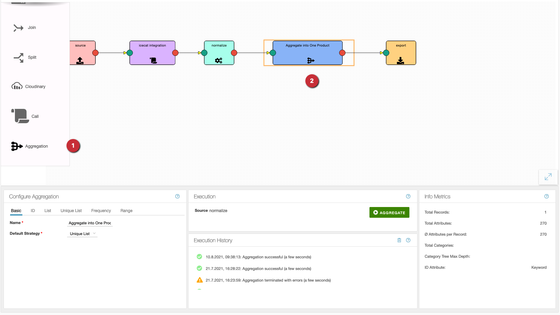
- As usual, the operation can be dragged from the left column onto the workspace.
- After that, the aggregation is connected to the desired flow elements.
There are 6 tabs to configure the aggregation:
Basic
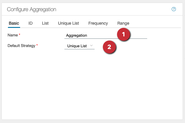
- A meaningful name for the aggregation should be assigned
- The following settings are possible for ‘Default Strategy’: ⋅⋅* Lists, here all data are summarized without change ⋅⋅* Unique lists, here the data are taken over once, duplicates are not taken into account ⋅⋅* Frequencies behave like unique lists, additionally the frequency of occurrence is added The settings in this tab apply to the whole operation.
ID
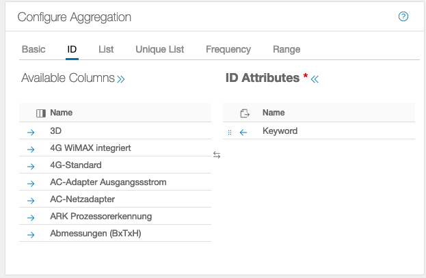
This declares an attribute to be an ID. There must be at least one ID attribute.
List
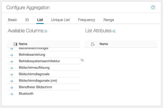
The data is summarized without change.
Unique List
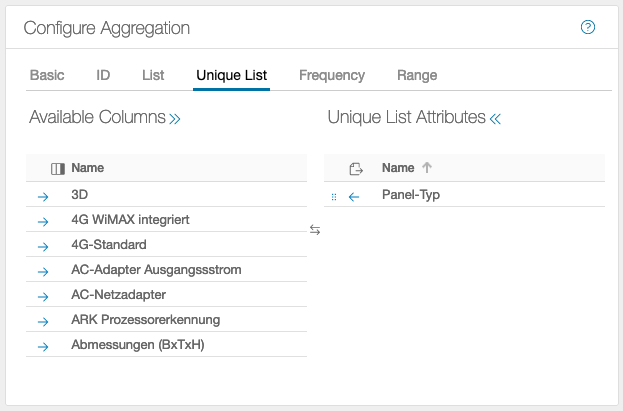
Here the data is taken over once, and duplicates are not taken into account. To determine the number of duplicates, the Frequencies tab is used.
Frequency
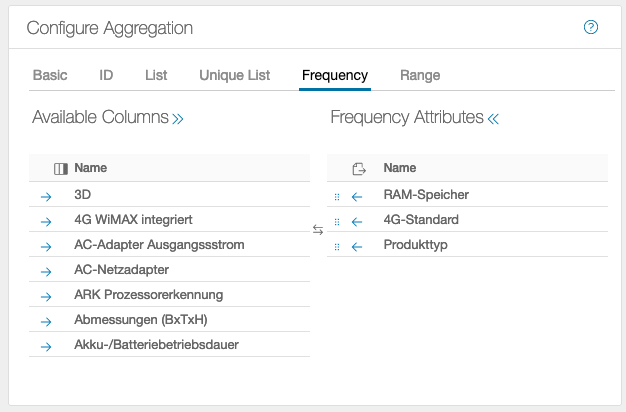
In the example, the frequencies of the attributes RAM, 4G and type are returned, i.e. the data is accepted once, and the frequency is incremented for a further occurrence.
Range
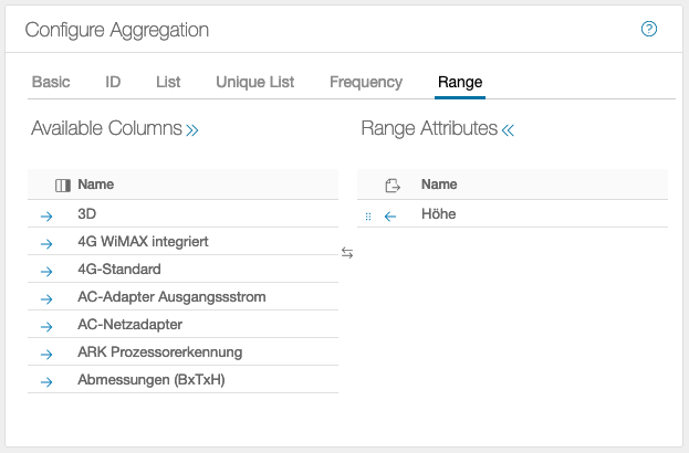
In this example, the Height column is evaluated. The minimum and maximum heights are returned as the result. The Ranges tab can only be used on numeric data, all other values will result in an error.